IEEE Signal Processing Cup 2021

Configuring an Intelligent Reflecting Surface for Wireless Communications

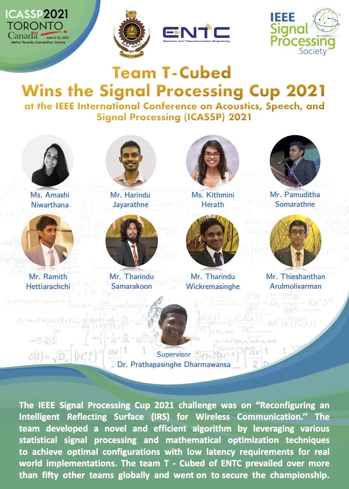
🏆 Grand Prize Winner: 1st place in the final round of the IEEE Signal Processing Cup 2021 · University announcement · ▶ Watch the final presentation

In one line: a fast, simple and explainable algorithm that learns a wireless channel from a few pilot measurements and then configures a 4096-element intelligent reflecting surface to maximise each user’s data rate. It runs in about a second on a Raspberry Pi 4 and reaches 99% of the data rate of our slower, high-precision mode.

---

At a glance

🏆 Result	Grand Prize Winner (1st place): one of three finalist teams that presented at ICASSP 2021, and the winner of the final round
Competition	IEEE Signal Processing Cup 2021, presented at ICASSP 2021
Challenge	Characterise an intelligent reflecting surface (IRS) from over-the-air signals, then control it to improve wireless communication for line-of-sight (LOS) and non-line-of-sight (NLOS) users
Our approach	Linear channel model with least-squares estimation, dimensionality reduction using the channel’s periodic structure, and a configuration search combining a genetic algorithm with gradient descent
Headline results	99.14 % of precision-mode data rate in fast mode · 340 ms per user on a laptop · 1.3 s on a Raspberry Pi 4
Two modes	Fast mode (genetic algorithm only) and precision mode (genetic algorithm + gradient descent)
Tech	Linear regression · genetic algorithm · gradient descent (Adam, Lookahead) · Raspberry Pi 4

---

The challenge

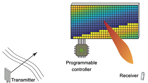
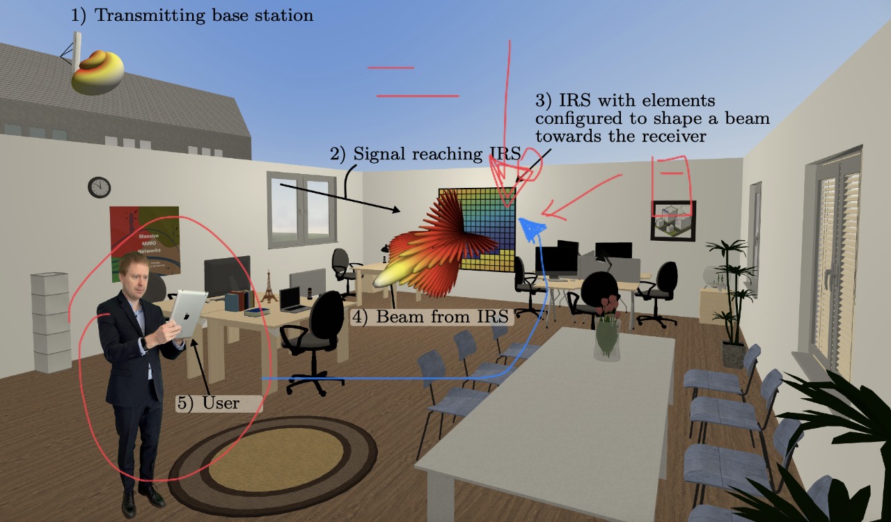
An intelligent reflecting surface is a panel made of many small elements whose reflection can be switched. By choosing the state of every element, the panel can steer a radio signal towards a user, boosting their data rate without any extra transmit power.

In this competition the IRS had 4096 elements, each in one of two states (+1 or −1). The goal of the challenge was to characterise the behaviour of the surface from signals recorded in an over-the-air signalling phase, and then develop a control algorithm that configures the surface to aid wireless communications.

Our task had two parts:

1. Estimate the channel. Model both the controllable channel (the path through the IRS) and the uncontrollable channel (all the paths that bypass it).
2. Search for the best IRS configuration for each user, whether LOS or NLOS, so that their received data rate is as high as possible.

Dataset 1	Plenty of measurements for a single user. We used it to understand the system
Dataset 2	50 users with only a limited number of pilot measurements each. Our algorithm had to work here

What made it hard

Challenge	Why it is hard	What we did
Unknown channel properties	Most physical details of the IRS and its surroundings were not given	Inferred noise level and channel structure from Dataset 1
LOS vs NLOS users	Do they need separate models?	One model works for both, so the pipeline is user independent
Too few pilots	About 4097 unknowns per tap but far fewer data points	Exploited the channel’s periodic structure to cut that to 65
Binary search space	2^4096 configurations, and a discrete space has no gradients	Relaxed to a continuous space, and used a gradient-free genetic algorithm
Non-convex objective	Gradient descent gets stuck in local minima	Used the genetic algorithm to warm-start and to escape local minima
Real-time, simple hardware	The result must be ready within a practical coherence time	Enforced periodic patterns so the search converges in milliseconds

---

Our approach

1. Channel estimation

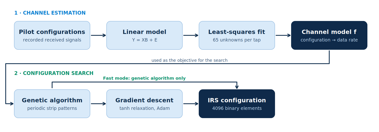
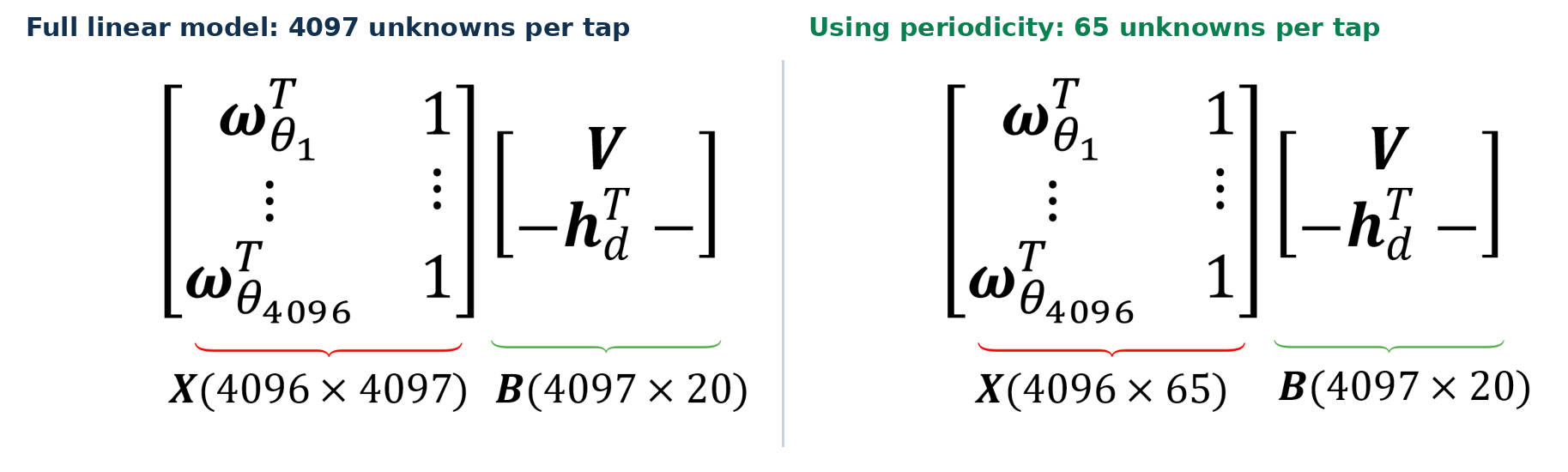
We model the system as a linear model, Y = XB + E, where Y holds the received signals, X holds the pilot IRS configurations, and B holds the channel we want to estimate. B contains both the controllable channel V and the uncontrollable channel h_d. With Gaussian noise, the maximum-likelihood estimate is the least-squares solution B̂ = (XᵀX)⁻¹XᵀY.

Dataset 1 gave us three useful observations:

• The noise is well described as Gaussian, and its variance could be measured.
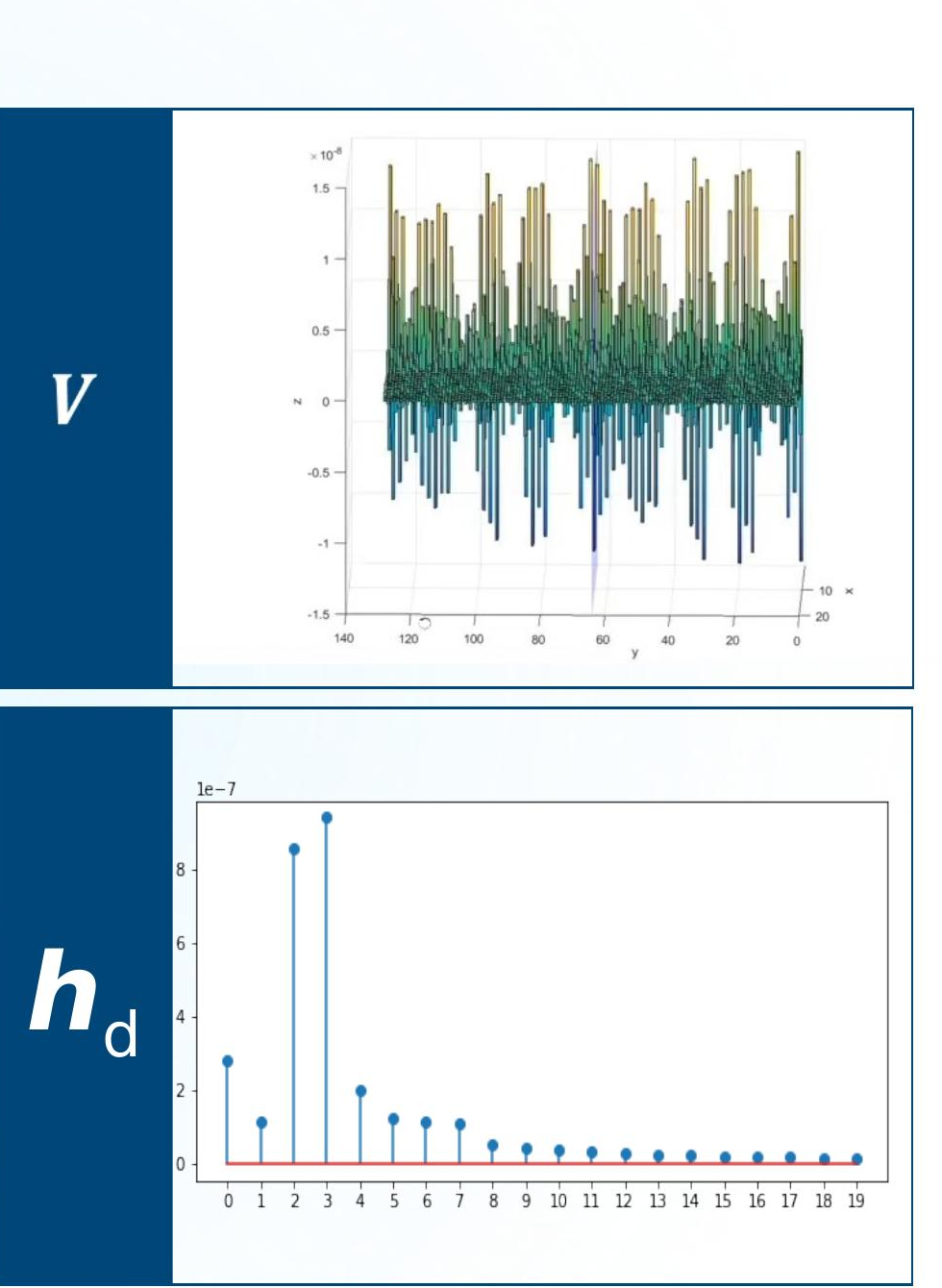
• Each tap of V is periodic with period 64, which supports the idea that the IRS is a square 64 × 64 grid.
• h_d looks like a typical multipath fading channel, so it matters for NLOS users and must be estimated accurately along with V.

With the limited pilots of Dataset 2, the full model has more unknowns than data points. Using the periodicity of V (following the spatial channel model of Björnson and Sanguinetti), we reduced the unknowns from 4097 to 65 per tap. The result is a simple, well-posed least-squares problem that works the same way for LOS and NLOS users.

2. Configuration search

Once the channel is estimated, we have a function f that maps any IRS configuration to the received data rate. We then need to search for the best configuration. We tried and combined two ideas.

	Gradient descent	Genetic algorithm
Idea	Relax the binary states to a continuous space, then follow gradients	Evolve a population of configurations with crossover and mutation
Strengths	Fine-grained, precise improvements	Gradient-free, very fast, handles binary variables naturally
Weaknesses	Slow and heavy on hardware, and gets stuck in local minima	Fast but only reaches a good sub-optimum

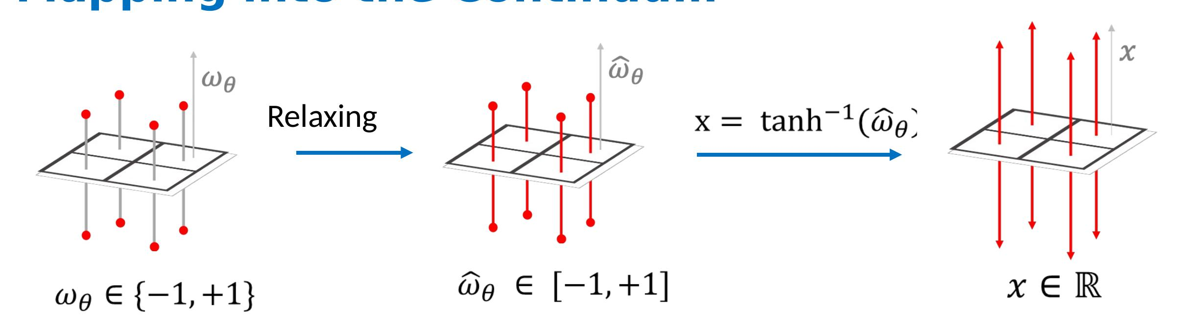
Gradient descent on a relaxed space. Each element’s state is relaxed from {−1, +1} to [−1, +1] and then mapped to the whole real line through a tanh activation. This lets us define a cost function from the data-rate function and optimise it with the Adam and Lookahead optimisers. The final configuration is obtained by discretising the result.

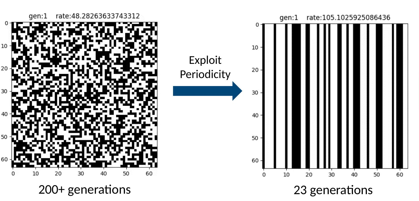
A genetic algorithm that exploits periodicity. A naive genetic algorithm mutates every element independently. We noticed that vertical-strip patterns give higher data rates, so we enforced that periodic structure. The search converges in 23 generations instead of 200+, which takes it from minutes to milliseconds.

Combining both. The genetic algorithm gives a fast, good starting point, which we use as a warm start for gradient descent. If more time is available, the two can alternate, and a mutation in the genetic algorithm can help escape a local minimum.

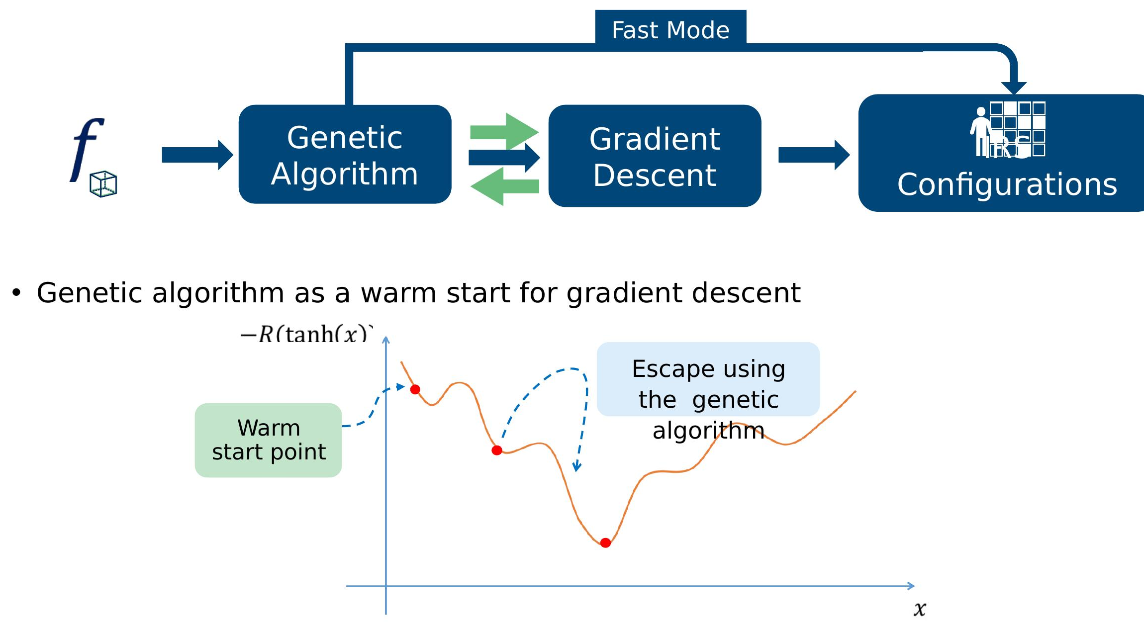
Mode	Search steps	When to use it
Fast mode	Genetic algorithm	Real-time use on simple hardware
Precision mode	Genetic algorithm, then gradient descent	A little more data rate for more time
Extended	Genetic algorithm, gradient descent, genetic algorithm, …	Squeeze out more data rate with more compute

---

Results

Mode	NLOS average (Mbps)	LOS average (Mbps)	Weighted average (Mbps)	Average execution time
Fast mode	63.54	115.15	118.49	340 ms
Precision mode	63.94	116.27	119.52	5 min

Data rates are measured against our own channel estimate. Execution time was measured on an Intel Core i5-8257U laptop.

Fast mode reaches 99.14 % of the precision-mode data rate and is roughly 800× faster. That is the trade-off that makes the solution practical.

Running on simple hardware

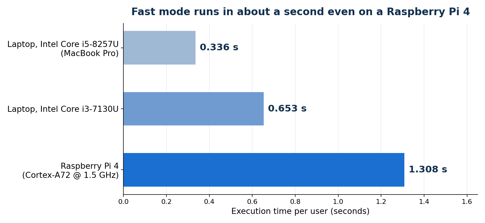
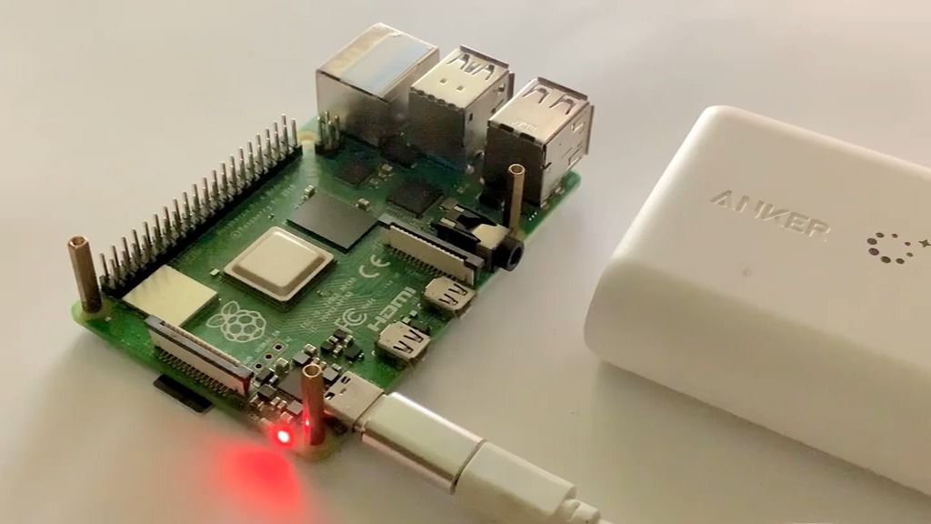
The whole pipeline, channel estimation and configuration search for one user, was tested on a Raspberry Pi 4 and on two ordinary laptops:

Device	Processor	Execution time
Raspberry Pi 4	Broadcom BCM2711, quad-core Cortex-A72 (ARMv8) @ 1.5 GHz	1.308 s
Laptop (MacBook Pro)	Intel Core i5-8257U, 1.4 GHz quad-core	0.336 s
Laptop	Intel Core i3-7130U, 2.70 GHz	0.653 s

These runs achieve about 98 % of our submitted results.

---

Recognition

🏆 Team T-Cubed won the Grand Prize (1st place) at the IEEE Signal Processing Cup 2021.

The SP Cup is an annual IEEE Signal Processing Society competition in which undergraduate teams solve a real-world problem with signal processing. The three best teams from the open competition are invited to present in a final round at ICASSP, the society’s flagship conference. In 2021 that final was held virtually, and our team won it. The University of Moratuwa’s announcement describes the winning work as a novel and efficient algorithm that reaches optimal configurations within the low-latency requirements of real-world use. Read the announcement.

---

Why it works

• Simple and explainable. Every step is a well-known method chosen for a reason. There are no black-box models or unexplained parameters.
• Works with limited data. Using the channel’s structure leaves only a few unknowns to estimate.
• One pipeline for every user. The same model and search handle LOS and NLOS users.
• Practical. Milliseconds on a laptop and about a second on a Raspberry Pi 4, with two modes to trade speed against data rate.

---

Conclusions

• A simple yet effective solution built from carefully chosen, well-understood algorithms.
• Two variants: a fast mode that gets 99 % of the data rate within milliseconds on simple hardware, and a precision mode for slightly higher rates.
• Practical to deploy, with the entire process needing minimal time and hardware.
• A user-independent pipeline that handles both LOS and NLOS users.

---

Team and acknowledgements

• Team T-Cubed: A. Niwarthana, H. Jayarathne, K. Herath, P. Somarathne, R. Hettiarachchi, T. Samarakoon, T. Wickremasinghe, T. Arulmolivarman
• Supervisor: P. Dharmawansa
• Department of Electronic & Telecommunication Engineering, University of Moratuwa, Sri Lanka

References

• E. Björnson and L. Sanguinetti, IEEE Wireless Communications Letters, 2021 (spatial channel model used for the channel estimation).
• E. Björnson, H. Wymeersch, B. Matthiesen, P. Popovski, L. Sanguinetti and E. de Carvalho, “Reconfigurable Intelligent Surfaces: A Signal Processing Perspective With Wireless Applications,” 2021.